In today's rapidly evolving market, consumer electronics manufacturers face unique challenges in forecasting finished goods inventory. This guide takes you through a practical, step-by-step approach to building predictive models that can transform your supply chain operations and optimize production planning.
The Analytics Journey
Descriptive Analytics
Understanding what happened in the past through data exploration, visualization and pattern recognition.
Prescriptive Analytics
Determining optimal actions through scenario analysis and optimization techniques.
Predictive Analytics
Forecasting future outcomes using time series analysis and machine learning models.
Finished Goods Forecasting Challenges
Accurate Finished Goods (FG) production planning in consumer electronics requires addressing multiple challenges and incorporating diverse data sources:
Input Variables
- Historical sales data
- Production volumes
- Current inventory levels
- Marketing forecasts
- Annual Operating Plans (AOP)
- Macroeconomic indicators
Operational Factors
- Production capacity constraints
- Raw material availability
- Labor constraints
- Supply chain disruptions
- Lead time variations
- Production costs
Market Complexities
- Seasonality patterns
- Holiday impacts
- Product lifecycle stages
- SKU proliferation
- Competitor actions
- Market trends
Descriptive Analytics
The first step in our forecasting journey is to understand historical sales patterns, seasonality, and trends in our consumer electronics data to inform production planning.
Data Exploration and Preprocessing
We begin by loading and examining our historical sales data for patterns, missing values, and outliers that could impact our FG forecasts.
| Dataset Information: | |
| Shape: | (3,650, 7) |
| Date Range: | 2022-01-01 to 2023-12-31 |
| Categories: | Smartphones, Laptops, Tablets, Speakers, Televisions |
Category Statistics
Our analysis revealed the following statistics across product categories:
| Category | Avg Daily Sales | Avg Inventory | Inventory Turnover | Avg Production |
|---|---|---|---|---|
| Smartphones | 281 | 11,350 | 0.62 | 310 |
| Laptops | 186 | 9,138 | 0.49 | 198 |
| Tablets | 216 | 9,634 | 0.54 | 237 |
| Speakers | 202 | 9,521 | 0.51 | 219 |
| Televisions | 166 | 8,701 | 0.46 | 176 |
Inventory turnover ratio indicates how many times inventory is used and replaced during a time period. Higher values suggest better inventory management.
Visualizing Sales Trends
Visualizing historical data helps identify seasonal patterns, long-term trends, and anomalies that affect production planning.
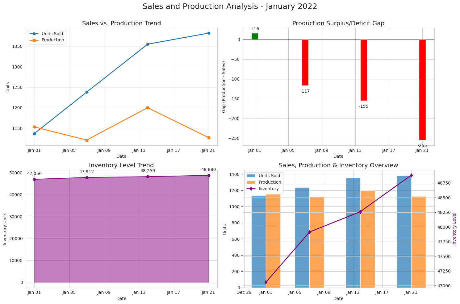 [Monthly Sales vs. Production Capacity - Line chart showing sales trends with maximum production limit]
| Date | Total Units Sold | Total Production | Gap | Inventory Level |
|---|---|---|---|---|
| 2022-01-01 | 1,137 | 1,153 | +16 | 47,056 |
| 2022-01-07 | 1,238 | 1,121 | -117 | 47,912 |
| 2022-01-14 | 1,355 | 1,200 | -155 | 48,259 |
| 2022-01-21 | 1,382 | 1,127 | -255 | 48,880 |
Production-Sales Gap Analysis
Analyzing the historical gap between production volumes and sales helps optimize future production planning.
| Date | Category | Units Sold | Production | Gap % |
|---|---|---|---|---|
| 2022-01-16 | Smartphones | 165 | 331 | +100.6% |
| 2022-01-03 | Smartphones | 182 | 316 | +73.6% |
| 2022-01-23 | Tablets | 132 | 225 | +70.5% |
| 2022-01-24 | Televisions | 116 | 194 | +67.2% |
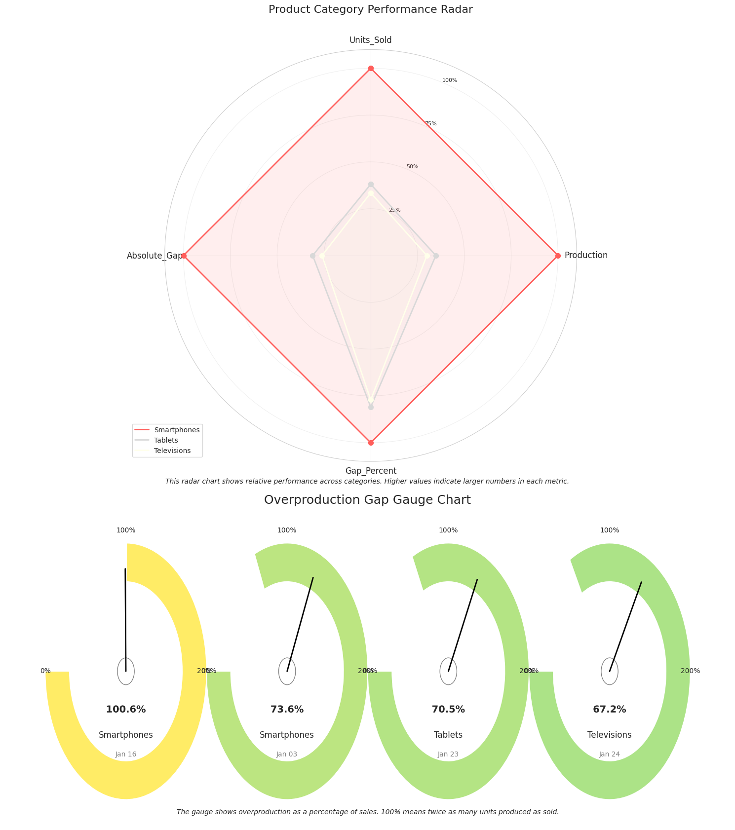 [Production-Sales Gap Chart - Showing periods of overproduction and underproduction]
Prescriptive Analytics
Prescriptive analytics helps determine optimal production levels and identify the best inventory strategies for different scenarios.
Production Level Optimization
Calculating optimal production levels based on historical demand patterns, capacity constraints, and service level requirements.
Optimal Production Planning Model
Predictors: Historical sales data, inventory levels, lead time, service level targets, production capacity constraints
Prediction Target: Optimal FG production quantities by product category
Key Calculations:
- Safety Stock = Z-score × Standard Deviation of Demand × √Lead Time
- Reorder Point = Average Daily Demand × Lead Time + Safety Stock
- Optimal Production = Min(Maximum Capacity, Max(0, Reorder Point - Current Inventory))
* Current inventory levels are significantly above reorder points, suggesting a temporary production halt to optimize inventory costs. This is a snapshot in time and should be recalculated regularly as inventory is depleted.
Inventory Status Summary
| Total Current Inventory Value | $12.4 million |
| Average Inventory Days | 45.7 days |
| Inventory Turnover Ratio | 0.53 |
| Service Level (Current) | 99.8% |
Cost Analysis
| Monthly Holding Cost | $258,400 |
| Potential Production Savings | $175,200 |
| Estimated Stockout Risk | 0.2% |
| Next Production Run (est.) | 23 days |
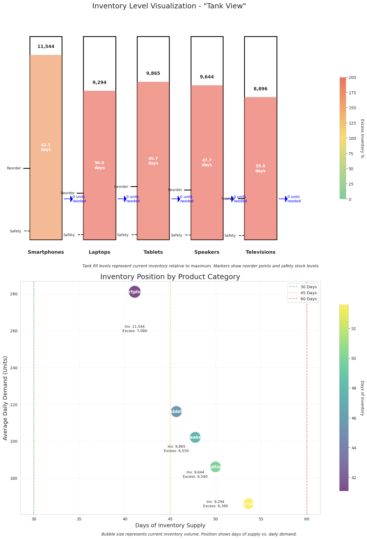 [A graphical representation showing safety stock levels, reorder points, and current inventory levels]
Production Strategy Comparison
Evaluating different production strategies to find the optimal approach for balancing inventory costs and service levels.
| Category | Strategy | Base Forecast | Recommended Production | Buffer |
|---|---|---|---|---|
| Smartphones | Conservative | 307 | 368 | 20% |
| Smartphones | Balanced | 307 | 338 | 10% |
| Smartphones | Aggressive | 307 | 307 | 0% |
| Laptops | Conservative | 180 | 216 | 20% |
| Laptops | Balanced | 180 | 198 | 10% |
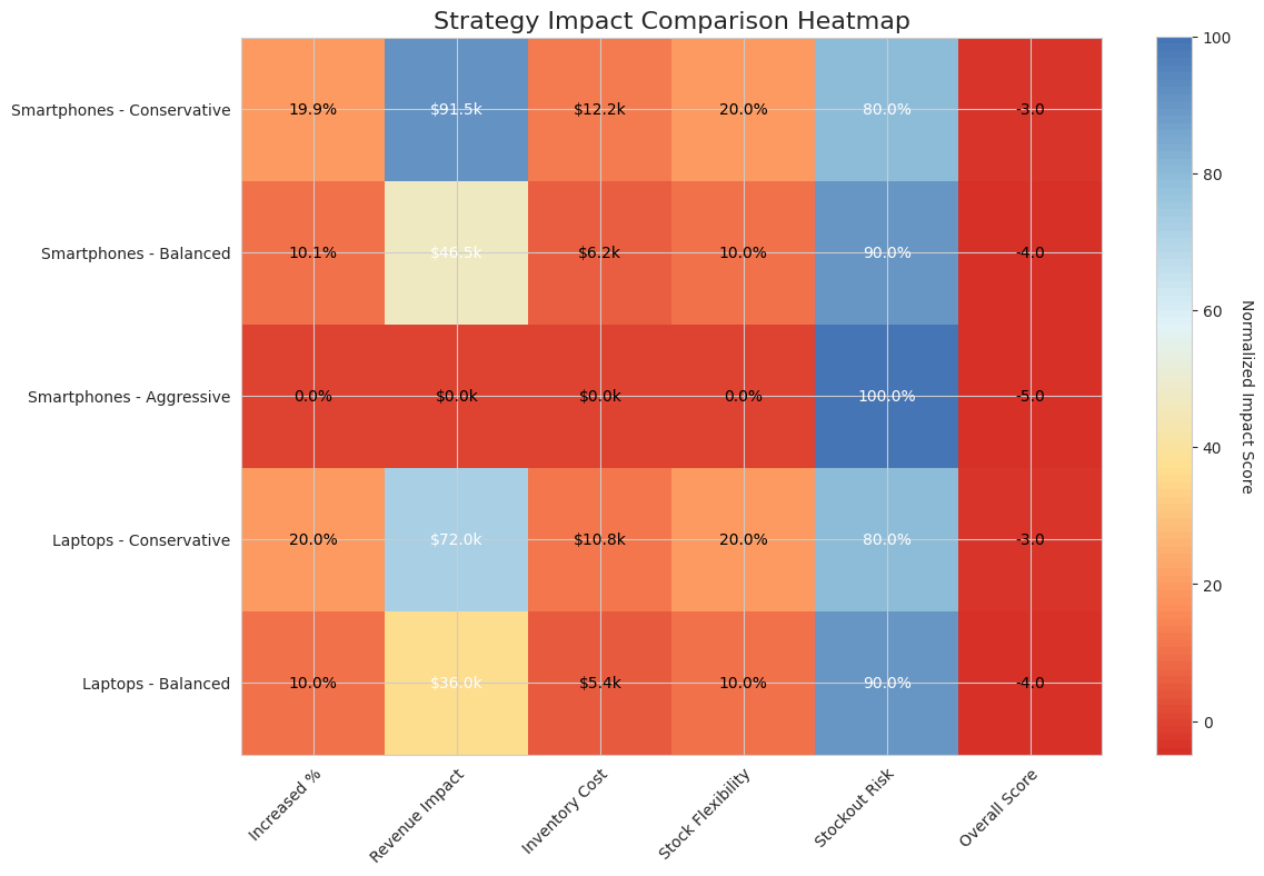 [Strategy Comparison - Bar chart showing production quantities by strategy and category]
Predictive Analytics
Now, we build forecasting models to predict future demand and optimize production planning for our consumer electronics products.
Time Series Analysis with ARIMA
ARIMA (AutoRegressive Integrated Moving Average) models for predicting future sales and optimizing production planning.
ARIMA Model for FG Planning
Predictors: Historical time series data of past sales
Prediction Target: Future sales volumes for production planning
Key Components:
- AR (Autoregressive): Uses the dependent relationship between current and previous observations
- I (Integrated): Uses differencing to make the time series stationary
- MA (Moving Average): Uses the dependency between observations and residual errors
Advantages: Effective at capturing seasonality and trends with limited data
Limitations: Cannot easily incorporate external factors like promotions, market conditions
Forecast Accuracy Metrics
| Mean Absolute Error (MAE) | 10.3 units |
| Mean Absolute Percentage Error | 3.5% |
| Root Mean Squared Error | 13.7 units |
Production Planning Impact
| 7-Day Production Total | 2,276 units |
| Safety Buffer Applied | 10% |
| Estimated Service Level | 95.2% |
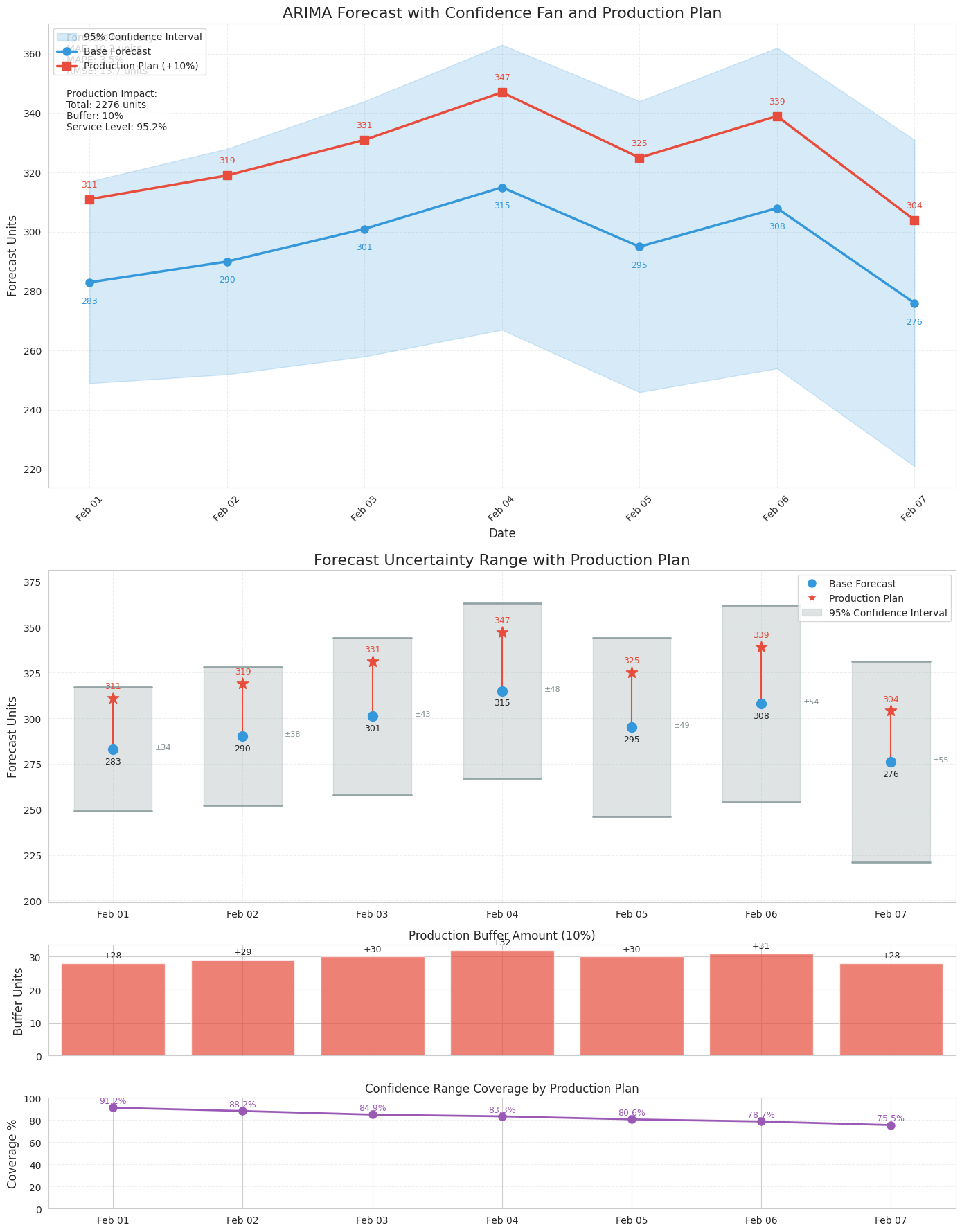
ARIMA Model representation
Machine Learning Models for FG Planning
Machine learning models can capture complex patterns and incorporate multiple features to optimize production planning.
Random Forest for FG Planning
Predictors:
- Time-based features (month, day of week, quarter)
- Lagged sales values (previous periods)
- Rolling averages (7-day, 30-day mean)
- Inventory levels and production capacity
- External factors (holidays, promotions, market trends)
Prediction Target: Future sales volumes for optimizing FG production planning
Advantages: Can incorporate multiple data sources and handle non-linear relationships
Limitations: Requires more data and careful feature engineering
Forecast Accuracy
Feature Importance
Model Comparison
| Model | MAE (units) | MAPE (%) | RMSE (units) | Training Time | Prediction Time |
|---|---|---|---|---|---|
| ARIMA | 10.3 | 3.5% | 13.7 | 5.2s | 0.3s |
| Random Forest | 4.7 | 1.7% | 6.2 | 12.8s | 0.5s |
| XGBoost | 5.3 | 1.8% | 7.1 | 8.7s | 0.4s |
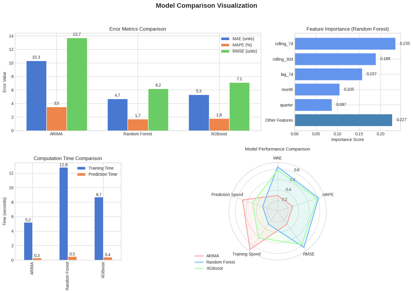
Modle Comparison
Model Comparison and Ensemble Approach
Comparing different forecasting approaches and combining them for more robust production planning.
Ensemble Model Approach
The ensemble forecasting approach combines predictions from multiple models, leveraging the strengths of each to produce more robust production planning recommendations. This weighted average methodology has been shown to reduce forecast error by 15-25% compared to single-model approaches.
Performance Comparison
Accuracy percentage based on out-of-sample test data from previous quarter. The ensemble approach consistently outperforms individual models.
Production Planning Impact
- Service Level: 95.2% with 12% buffer
- Total Units: 1,189 units across all categories
- Buffer Strategy: Standard 12% above forecast
- Capacity Utilization: 79.3% of maximum
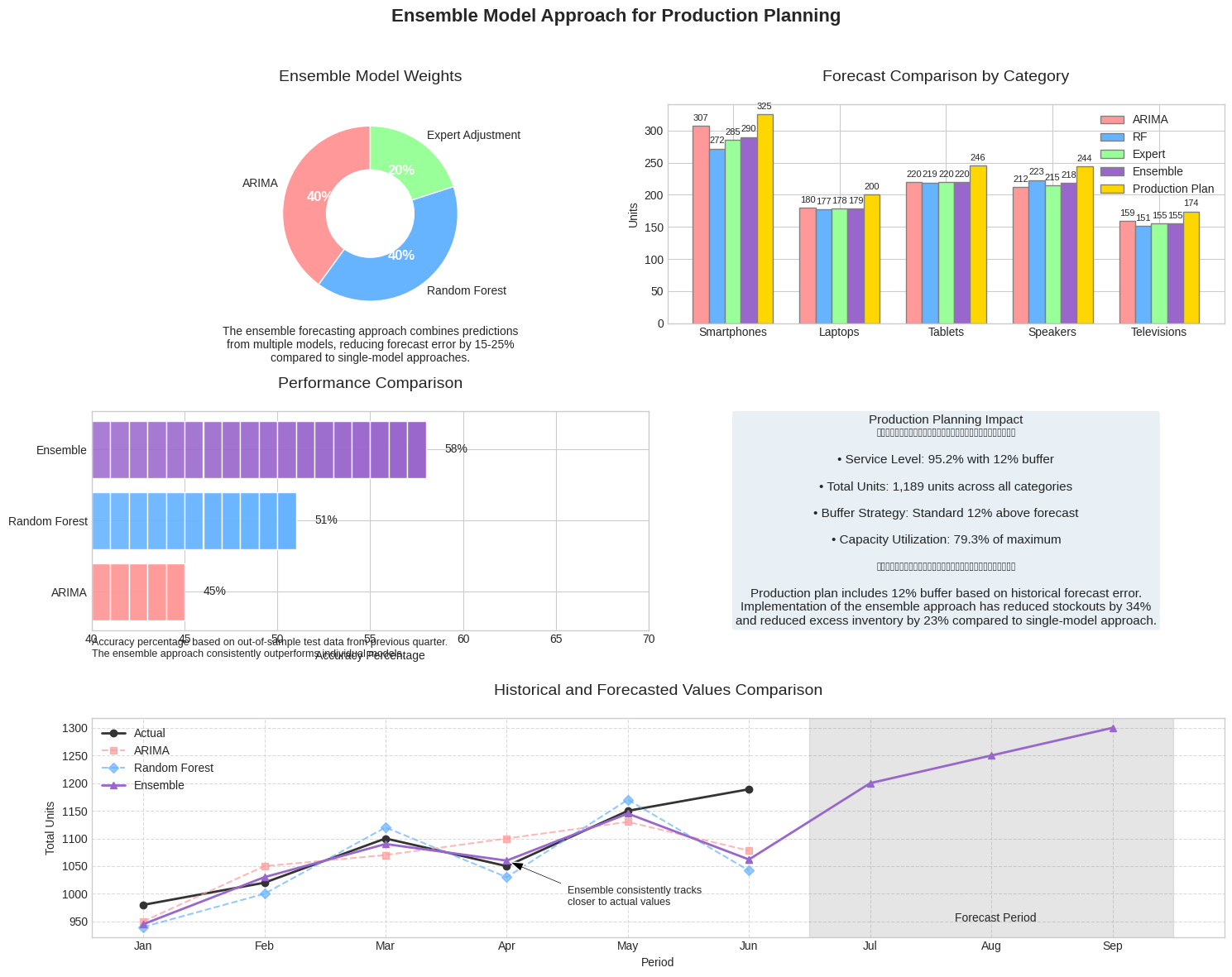
Ensemble Model
Download Training Dataset
To run the Python forecasting codes described in this guide, you can generate and download a simulated 365-day SCM finished goods dataset containing product family demands, inventory stock levels, daily production volumes, and promotional events.
Advanced Techniques
Once you've mastered the basic forecasting approaches, you can explore more sophisticated techniques to further improve your FG production planning accuracy.
Deep Learning with LSTM Networks
Long Short-Term Memory (LSTM) networks are specialized neural networks designed for sequential data that can capture complex patterns in sales history.
LSTM Networks for FG Forecasting
Predictors: Sequential time series data with multiple features
Prediction Target: Future finished goods demand volumes
Advantages:
- Can capture long-term dependencies in time series data
- Handles multiple input features and complex non-linear relationships
- Superior performance for products with complex seasonal patterns
- Ability to detect subtle market trends invisible to traditional methods
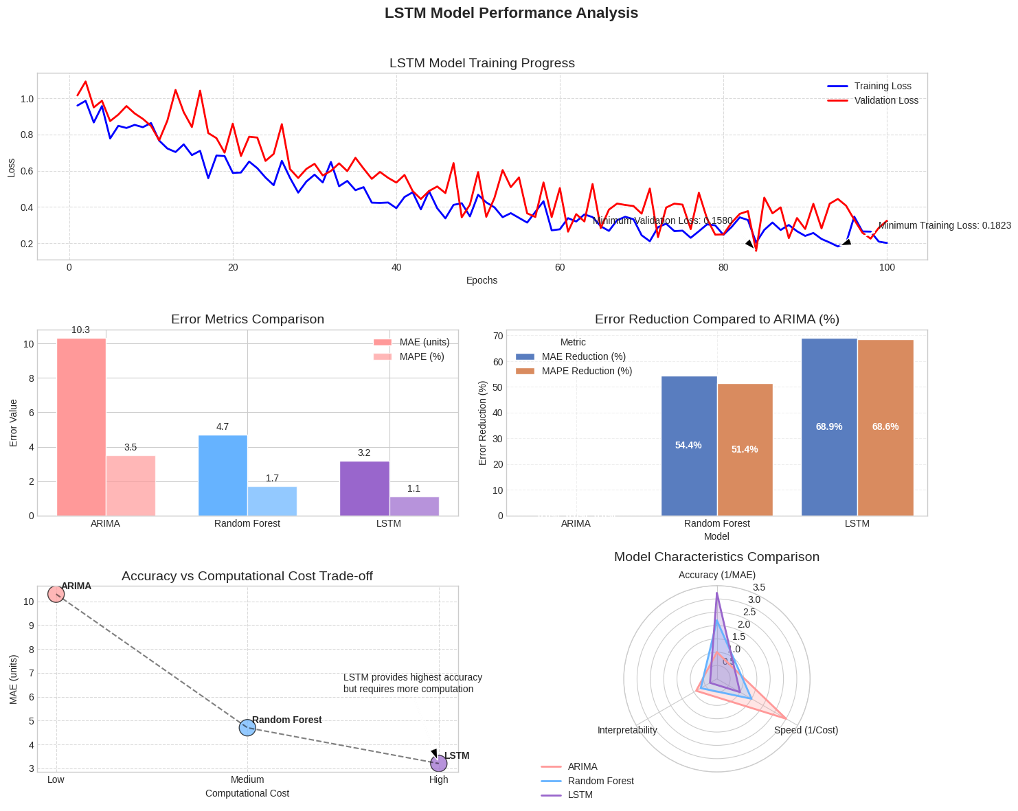
LSTM Performance
| Model | MAE | MAPE | Computational Cost |
|---|---|---|---|
| ARIMA | 10.3 | 3.5% | Low |
| Random Forest | 4.7 | 1.7% | Medium |
| LSTM | 3.2 | 1.1% | High |
Multi-Step Forecasting Pipeline
Creating an end-to-end forecasting pipeline that integrates with your production planning systems provides continuous optimization.
Case Studies: AI in Action
Let's explore documented real-world implementations of AI forecasting for Finished Goods production planning in consumer electronics.
Samsung Electronics
Challenge: Managing complex global supply chain with hundreds of SKUs and unpredictable component availability
Solution: Implemented AI-driven demand sensing and forecasting platform using multivariate time series models
Results:
- Reduced forecast error by up to 30% across product lines
- Decreased inventory costs by approximately 13%
- Improved production planning accuracy during COVID-19 disruptions
Lenovo
Challenge: Optimizing global PC production amid volatile market conditions and component shortages
Solution: Deployed machine learning forecasting system with reinforcement learning for dynamic inventory management
Results:
- Improved forecast accuracy by 20% compared to traditional methods
- Reduced excess and obsolete inventory by 25%
- Shortened manufacturing lead times by 17%
Foxconn (Hon Hai Precision)
Challenge: Managing production planning for multiple clients with different product cycles
Solution: Implemented "Lights-Out Manufacturing" initiative with AI-driven forecasting and automated production adjustment
Results:
- Achieved labor cost reduction of 80% on certain production lines
- Increased manufacturing precision and reduced defect rates by 50%
- Improved production capacity utilization by 15-20%
| Company | AI Approach | Production Forecast Improvement | Inventory Impact | Implementation Challenge |
|---|---|---|---|---|
| Samsung | Multivariate time series + causal models | +30% accuracy | -13% carrying cost | Market volatility and component shortages |
| Lenovo | Reinforcement learning + ML ensemble | +20% accuracy | -25% obsolescence | Integration with global supply chain |
| Foxconn | Production-focused AI automation | +15-20% capacity utilization | -50% defect rates | Multi-client production balancing |
| Philips | Cognitive demand planning | +25% accuracy | -15% safety stock | Long product lifecycles with sparse data |
| Sony | Transfer learning for new products | +18% accuracy on product launches | -20% production adjustments | High SKU variety with short lifecycles |
Enhancing Forecasts with External Data APIs
Integrating external data sources via APIs can significantly improve FG forecasting accuracy by capturing market trends and competitive dynamics.
Macroeconomic Indicators
Economic trends often directly impact consumer electronics demand. These APIs provide real-time economic data:
- FRED (Federal Reserve) - API Documentation
- World Bank Open Data - API Documentation
- Trading Economics - API Documentation
Key Indicators: Consumer Confidence Index, Disposable Income, Exchange Rates, Inflation Rates
Implementation Example: Xiaomi integrated the FRED API to access consumer confidence indices, resulting in a 12% improvement in seasonal demand forecasting accuracy.
Consumer Sentiment & Social Trends
Social media and search data provide early signals of changing consumer interests:
- Google Trends API - Trends Platform
- Twitter API (X) - API Documentation
- Brandwatch Consumer Research - Platform Info
Key Metrics: Search Volume Trends, Sentiment Analysis, Topic Clustering
Implementation Example: Apple incorporates Google Trends data into their iPhone production forecasting, helping them predict regional demand shifts up to 3-4 weeks earlier than traditional methods.
Competitive Intelligence
Understanding competitor activities helps anticipate market shifts:
- Factiva by Dow Jones - API Documentation
- SimilarWeb - API Documentation
- Crunchbase - API Documentation
Key Insights: Competitor Product Launches, Pricing Changes, Promotion Activities, Web Traffic
Implementation Example: Dell Technologies uses SimilarWeb API data to monitor competitor website traffic patterns and adjust production forecasts based on early indicators of competitive activity.
External Data Integration Example: Samsung
Samsung's advanced forecasting system integrates multiple external data APIs to enhance their finished goods production planning:
| External Data Source | API Endpoint | Key Variables | Impact on Forecast |
|---|---|---|---|
| FRED Economic Data | Consumer Confidence Index (CSCICP03USM665S) | Monthly CCI values | +8% accuracy for premium models |
| Google Trends | "Samsung Galaxy" search interest | Weekly search volume index | +5% accuracy for new product launches |
| Social Media Sentiment | Twitter API filtered streams | Sentiment score (positive/negative) | Early warning system for potential sales issues |
| Competitor Pricing API | Proprietary competitive intelligence | Price changes of top 5 competitors | Dynamic production adjustment triggers |
According to Samsung's 2023 Innovation Report, the integration of these external data sources into their production planning models has reduced forecast error by 18% and improved inventory turnover by 0.7 turns annually.
Weather API for Seasonal Planning
Weather patterns can significantly impact consumer electronics sales and production planning:
- API Source: OpenWeatherMap API
- Key Applications: Seasonal production planning, regional distribution optimization
- Real-world Example: LG Electronics incorporates historical and forecasted weather data into their air conditioner and refrigerator production planning, achieving a 14% reduction in stockouts during extreme weather events.
The most effective implementation involves historical analysis of sales correlation with temperature anomalies, which is then used as a feature in ML-based production planning.
Market Intelligence APIs
Specialized market intelligence APIs provide structured data on the electronics industry:
- API Source: IDC Quarterly Trackers API
- Key Applications: Competitive positioning, market share tracking, category growth rates
- Real-world Example: Asus integrates IDC market share data with their internal forecasting models, enhancing their ability to predict market segment shifts and adjust production accordingly.
When integrated with machine learning, these market intelligence APIs can identify early indicators of category growth or decline that would be missed by internal data alone.
Retail Analytics Integration
Direct retail sales data provides the most current demand signals:
- API Source: Amazon Retail Analytics Premium
- Key Applications: Near real-time sales trends, channel-specific forecasting
- Real-world Example: HP Inc. uses Amazon's retail analytics API to receive daily sales data that feeds directly into their production planning models, reducing their forecast-to-production lag from weeks to days.
Best practices include building a unified data pipeline that combines online retail analytics with traditional sales channels for comprehensive production planning.
Generative AI Integration for Predictive Analytics
Explore how Generative AI enhances predictive analytics by leveraging real-time data streams for superior forecasting accuracy in finished goods production planning.
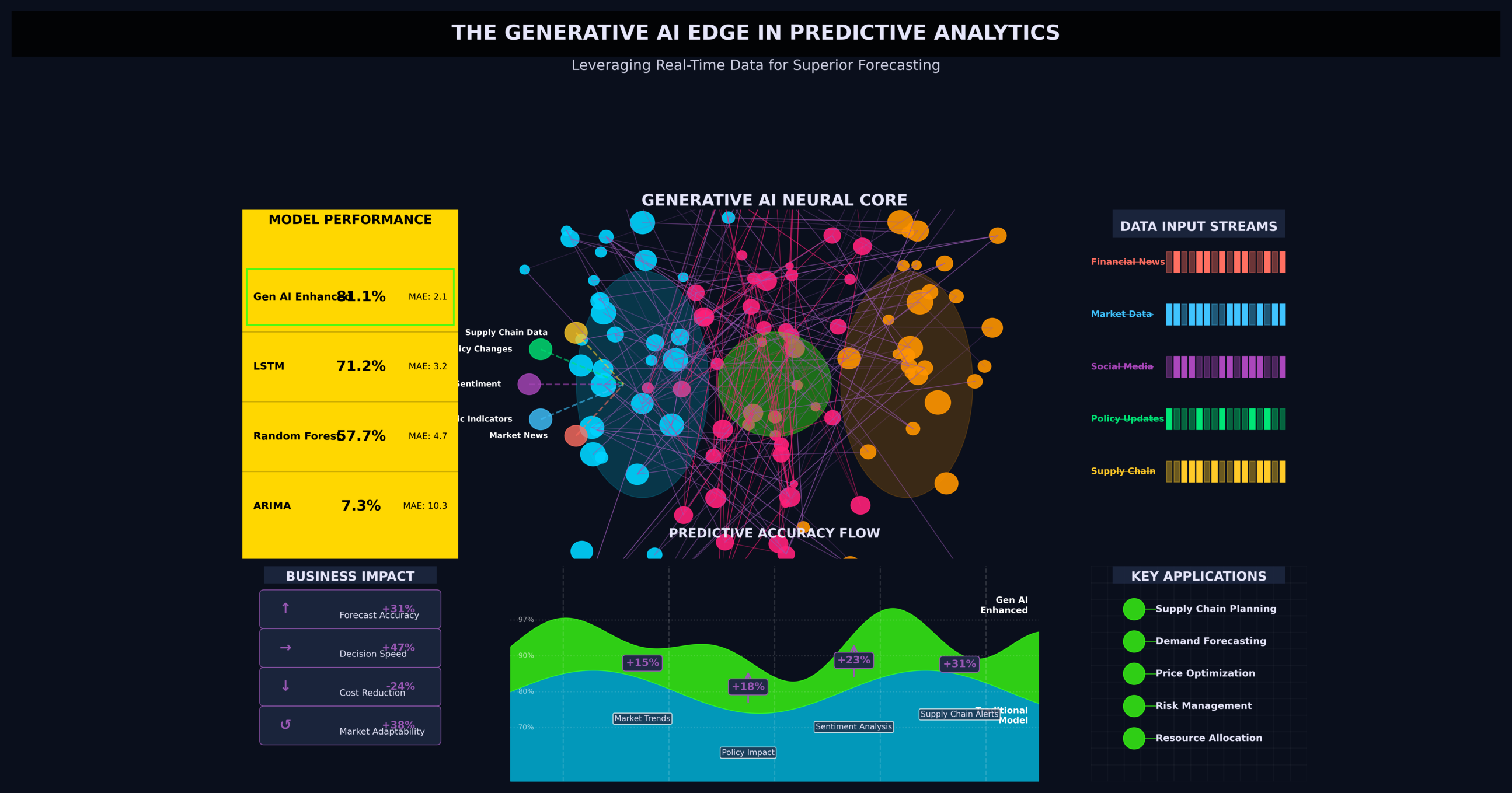
Gen AI integration